


The post-Double Time Android: Netrunner OCTGN dataset contains 211,854 games played since September 2012. There are a lot of ways to slice this data up and look at it, so to preface my own work I want to say thanks to dbzer0, Hollis, Alexfrog, Miaowara_Tomokato, Lysander, and the others who built the foundations of OCTGN data analysis. We’ve seen excellent work such as Hollis’ Balace at the 99th Percentile, Alexfrog and Captain_Frisk’s look at The Effect of Player Skill on Winrates, Miaowara_Tomokato’s analysis of the effect of player skill on flatline rates, and most recently, Lysander and Miaowara_Tomokato’s look at the Spin Cycle metagame.
I’ve been working on my own anlaysis for the last couple of months, looking at the last two ANR OCTGN datasets in numerous different ways as well as optimizing and refactoring my code. On that note, you can find the current version of the code I used to do all of this work (and more) here on GitHub. I’ll be updating it as I continue to work on ANR OCTGN analysis, so if you code in R and want to extend or improve it, awesome. Ideally, I will ultimately build it into an R package alongside a Shiny web app for interacting with the data.
Methodology
One disadvantage to starting at around the same time as everyone else is that I ended up duplicating a lot of work. Others have filtered the data, estimated player skill, and done flatline and faction winrate calculations, but I couldn’t build on their work for my analysis – it hadn’t been done yet. Since my methods differ slightly, I’ll give a quick overview of what I did.
First, I did some basic cleanup.
- Removed games where:
- Runner deck size was less than 45 cards.
- Corp deck size was less than 40 cards.
- Match duration was less than 0 minutes.
- Either player conceded.
- Removed invalid IDs:
- Laramy Fisk and The Collective.
- Jinteki and Haas-Bioroid: Selective Mind-Mapping.
- Removed games with missing data:
- Games with no version number (used to determine which data packs were valid).
Removing games with concessions is a brute force solution to the more complex problem of avoiding deliberate winrate inflation, but since very few games ended with concessions, I felt comfortable simply removing them rather than trying to filter legitimate concessions from people who conceded after a bad mulligan.
This left 167,760 games and 5,438 players. Like many others, I wanted to estimate player skill in a reliable way, so the next step was computing Glicko ratings for each player. The Glicko algorithm’s creator states that it works best when each player is playing 5-10 games in each rating period; after running Glicko calculations on the data for a couple of different periods, I chose to go with with weekly ratings for each player.
I like Glicko over ELO because in addition to the player rating estimate, it also provides an uncertainty measure called deviation. This is an indication of how confident we think we can be in a given player’s rating.
My initialization parameters were a 1500 rating and 350 deviation. After estimating the Glicko ratings for each player, my first plot of the distribution of Glicko ratings for the OCTGN data showed a number of peaks. There was a particularly large one around the default rating value, so I reasoned that this was likely attributatble to players who hadn’t played many games. If there were a lot of these players, then there should also be a high deviation shoulder in the distribution of deviations, and sure enough:
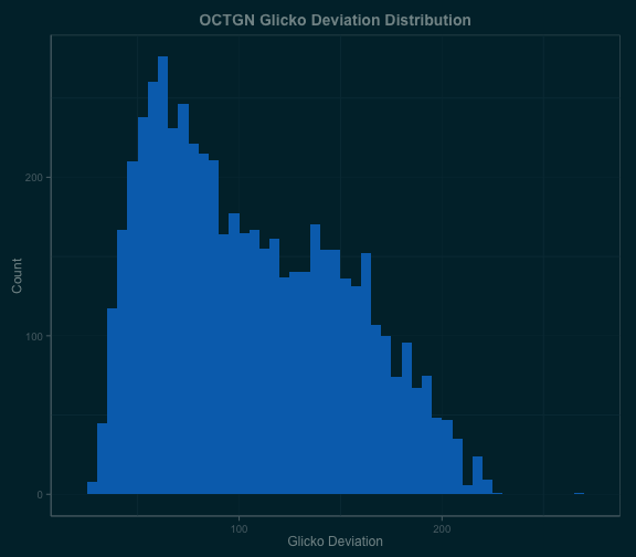
As expected, the high deviation shoulder overlapped with players who had played relatively few games, so I filtered out games where a player either had a Glicko deviation greater than 150 or had played fewer than 5 games. After that, I was left with a fairly normal distribution of player ratings:
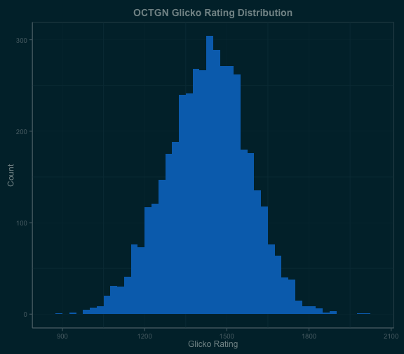
The average rating was 1428 and the standard deviation of the distribution was 149. To get a picture that could reasonably map to moderate-level tournament metas, I decided to limit the initial analysis to players rated higher than 1577 – i.e. more than one standard deviation above average. This left 678 players and 71,137 games in the dataset.
Finally, after doing all of this and looking at the data, I dropped the Double Time games, because there were simply too few of them. Overall, the faction winrates from this data were similar to previous “competitive cut” results… but that didn’t tell me anything new!
What Next?
I had a set of data containing games with fairly skilled players. What next? For a while, it seemed like every time I started to crunch through some analysis, someone else would write an article or start a BGG thread on the same topic. But there was one thing no one else was writing about: matchup data. Most of the work I’d seen focused on how a given faction or ID performed against the field in a specific set of circumstances: during a given data pack, say, or what share of their wins or losses came by flatline. But we had the data to look at how each Corp ID has performed against every single Runner ID over arbitrary periods of time, and vice versa. It’s just that no one had done it yet.
The next step was figuring out how to do it – but as it turned out, that was simple. dplyr is a new R package by one of the pillars of the R community, Hadley Wickham. It massively accelerates and simplifies precisely this type of grouping analysis, and as it happened I was already in the process of refactoring all of my code to leverage dplyr because of the huge performance gains. Using dplyr, the matchup winrate calculations were easy to implement and very fast to run, allowing me to spend a lot more time exploring the data and less time working on code.
It was clear from the data that the core IDs are played far more frequently on OCTGN than any of the non-core IDs, with the notable exceptions of Andromeda and Reina on the Runner side. Kit, the next most played Runner ID, has fallen off sharply since an initial surge of play.
On the Corp side, only the core four IDs have seen enough consistent play to exhibit meaningful trends. NBN: The World Is Yours and Jinteki: Replicating Perfection are close; TWIY has been seeing consistent play since True Colors, and RP is likely to pick up with the release of Honor and Profit. Cerebral Imaging has also seen a jump in play, but is still well below 100 games per matchup in recent data packs.
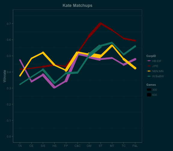
Shaper Matchups
Kate was the only Shaper played consistently enough for the analysis. On the matchup graph below, each line represents one of the core four Corp IDs, each point represents the release of a data pack (listed on the X-axis), and the thickness of the line is proportional to the number of games played in that matchup during that time frame. For example, Kate vs Weyland: Building a Better World was played 600+ times while Opening Moves was the latest data pack available on OCTGN.
Since there’s some overlap between matchup winrates, some may prefer to look at individual matchup plots. Those are shown below. The number of games in each period is at the top of the winrate bar.
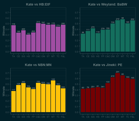
We’ve seen from Lysander’s analysis that Kate was more successful in the Spin Cycle than the Genesis Cycle. On the face of it, this seems obvious: Shapers gained a number of powerful tools, and many of the best synergize with Kate’s ability: Self-Modifying Code, Clone Chip, Scavenge, and Atman. All of these are good cards from Creation and Control, but Kate’s installation discount makes them just a little bit better; it’s no surprise that her winrate took off when Creation and Control was released.
However, from the matchup data, we can see that Kate’s biggest gains by far came against Jinteki: Personal Evolution, where she went from a mid-40s winrate during Future Proof all the way up to 70% by Second Thoughts. The cards I mentioned above are good versus PE by virtue of being good in every matchup, but Shaper also gained Levy AR Lab Access and Professional Contacts in Creation and Control. Both are strong cards, and both are particularly strong against PE.
NBN gained Wraparound in True Colors and Sweeps Week in Fear and Loathing; a winrate decline versus NBN: Making News over the course of those two data packs is a fairly common theme among the Runner matchups. Sweeps Week may be best versus Andromeda, but Shapers also draw plenty of cards thanks to Diesel and Quality Time.
Kate made a huge immediate gain versus Haas-Bioroid: Engineering the Future when Creation and Control was released, but the matchup hasn’t improved any further over time. As of Fear and Loathing, EtF is Kate’s second worst matchup behind MN in this skill bracket. I suspect that Atman was the biggest influence here because of how much of ETF’s typical ice loadout is either 4 or 5 strength – and since Atman decks haven’t gained anything for the EtF matchup since Atman itself was released, there has been no further change in winrate. Unfortunately, there’s no way to confirm this without deck lists in the OCTGN data.
It’s also interesting that Weyland: Building a Better World went from being Kate’s second worst matchup before Creation and Control to being her second best matchup by Fear and Loathing. This is a shift I don’t have an obvious explanation for; the cards I love to play against Weyland with my Kate Blitz deck – other than Plascrete Carapace – are Indexing (Future Proof) and Sharpshooter (True Colors). Power Shutdown and Accelerated Diagnostics were released in Mala Tempora, and Kate’s winrate vs BaBW did decrease somewhat after that, but she’s still winning comfortably above 50%. Also, BaBW’s other matchups don’t share the same trend, suggesting that there’s something unique about the Kate vs BaBW matchup for Weyland.
Next Steps
Initially, this will be a three-part series. Part 1 covered the methodology and Kate’s matchups; part 2 will cover Gabe, Andromeda, Noise, and Reina; part 3 will cover the four core Corp IDs. Even though the Corp data can be inferred by looking at the Runner data, I think it’s worth a separate discussion and generating similar plots for the Corp IDs, if only to summarize what we’ll have already seen on the Runner side.
Beyond that, the code I’ve written is only a starting point. Each time new OCTGN data is released, it will be simple to run all of the same analysis again and generate updated plots – all it requires is pointing the initial octgn.R script at a new data file, and unless the data format changes, it will work fine. If new elements are added to the OCTGN data, I or someone else can easily write a new script or modify octgn.R to make use of the new information.
Finally, my primary goal in doing all of this is to spark discussion. I do offer my own comments and opinions on possible reasons for the matchup winrate trends I observe in the data, but these are by no means definitive, and there are plenty of trends in the data that I have no clue how to explain. If you’ve got a great feel for how a particular matchup has shifted over time in your meta and can shed some light on the trends we see in the OCTGN matchup data, post about it! I love talking about Netrunner, and I think some of the best Netrunner discussion around happens here on Stimhack. I’m pretty excited to be contributing to the conversation.